This blog post was written by members of the GP2 Complex Disease Data Analysis working group.
In our last blog post, we gave an introduction to GWAS, including statistical formulae, workflows, and examples from the most recent Parkinson’s disease GWAS. Now we want to provide you with additional insights and tips for running your own GWAS.
Quality control and imputation processes
High quality genotypes (non-palindromic, i.e., no A/T, G/C if possible, with a high Illumina gentrain score indicating cluster quality) with low missingness ( < 1% per sample and per SNP is preferred).
Generally focus on common, minor allele frequency > 1%, any less and hope the genotype clusters look very good (you should inspect them).
Check samples for high rates of heterozygosity, as this could indicate potential contamination. Low rates of heterozygosity could also be problematic.
Be careful of duplicated samples and cryptically related samples.
Algorithmically ascertain and parse samples by genetic ancestry (we use a combination of fastStructure and flashPCA). Let’s maximize diversity but be wary of population substructure and its effects on the outcomes of analyses.
Look into SNPs that are not missing by chance, including bias due to missingness by case:control status or haplotype.
There is no reason you can’t use multiple imputation reference panels for a single population and use the resulting genotype with the best quality metric. This is particularly useful in admixed sample populations.
Tips on study level analyses
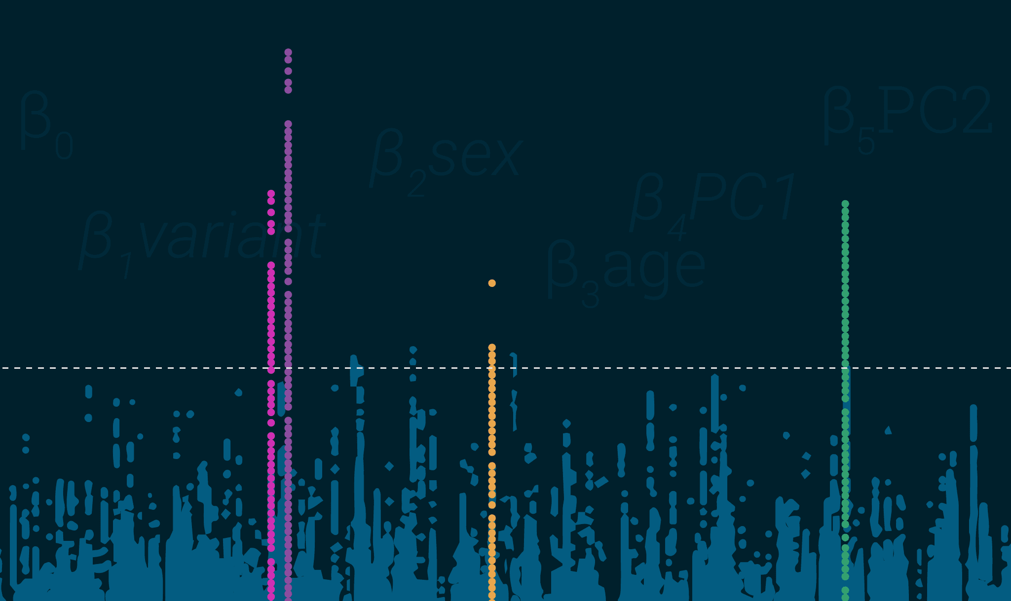
Regression – GWAS generally uses linear regression models for continuous outcomes and logistics for discrete outcomes. These quantify risk at an SNP while accounting for covariates.
A variety of software packages can be used to run mixed linear models, these models can accurately account for relatedness and fine scale population substructure.
PCs – Calculating principal component loadings based on genome-wide genotyping data makes a useful set of covariates for your regression models, effectively allowing you to account for population substructure.
Now let’s meta-analyze
Fixed vs. random – These are meta-analysis methods to combine data on a summary statistic level, across data silos and/or publications. Fixed effects meta-analyses are often useful for discovery analyses and generally more powerful, although some of us prefer random effects models as they are more conservative and account for heterogeneity across data silos.
Heterogeneity estimates – Often expressed as Cochrane’s Q or I2. Very important as they give an idea of outlier effect bias and generalizability of results.
Scrutiny results
Study level lambdas – keep it between 0.95 and 1.05, anything else and you have a problem.
Overall lambda and lambda 1000 – calculating lambdas on either the study level or the meta-analysis level can be tricky when you have a case: control imbalance. A massive excess of controls can artificially inflate the lambda statistic. In this case, use lambda1000 as it is scaled to 1000 cases and 1000 controls. Once again, code for this is in our GitHub repo.
Linkage disequilibrium (LD) score intercept – alternative / complement to lambda and more robust to LD structure and case: control imbalance.
LD peaks in plots showing uniformity – this is pretty straightforward, your results when plotted should look like towers in Manhattan (or your city of choice, sorry D.C.) not a snowstorm.
Replication – always good but sometimes you don’t have available datasets. When additional data is not available, try a combination of leave-one-out meta-analyses and cross-validation.
Some post-GWAS analyses
Or “what to do once your GWAS meta-analysis is complete”. Note that GP2 will be providing further blog posts and courses on these topics.
Conditional analyses – use the most significant SNP in a region as a covariate and rerun the analyses or use a tool like GCTA. You may have multiple independent signals per locus.
Fine mapping – This can be done through approximate Bayes factor analysis in packages like coloc including Bayesian colocalization (leveraging genomic reference data for gene expression or similar metrics).
Prediction weights and TWAS – A variety of packages exist to leverage external weights from gene expression, methylation, or chromatin studies, etc. to identify putative mechanistically connected genes hiding in your GWAS data.
ML – Purpose-built predictions, our favorite package is GenoML because it’s mostly automated and makes machine learning (ML) in genomics easy.
For more information, you can find our code and pipelines at the GP2 GitHub.
This blog was jointly authored by Hampton Leonard, Mike Nalls, Yeajin Song, and Dan Vitale. Please visit GP2’s Complex Disease – Data Analysis Working Group page to learn more about their background.